IMPORTANT:

Make sure to complete this hands-on lab on a desktop/laptop only.

There are only 5 attempts permitted per lab.

As a reminder – it is common to not get every question correct on your first try, and even to need to redo a task; this is part of the learning process.

Once a lab is started, the timer cannot be paused. After 1 hour and 30 minutes, the lab will end and you’ll need to start again.

For more information review the Lab technical tips reading.

Activity overview

Cloud data analytics is a rapidly evolving field, and cloud data analysts must continuously learn about new platforms and technologies to be effective in their jobs. Comparing different platforms, such as BigQuery and Dataproc, is a good way to do this.

BigQuery and Dataproc are both cloud data processing platforms, but they use different data processing engines, SQL dialects, and development environments to analyze data.

BigQuery is a data warehouse that is good for interactive queries on large datasets. It is easy to use and can handle a wide range of data analysis tasks.

Dataproc is a managed Hadoop and Spark service that is good for batch processing jobs on large datasets. It is more flexible than BigQuery, but it can be more complex to set up and use.

Both BigQuery and Dataproc are integrated with other Google Cloud services, making it easy to move data between them and to discover data lake sources.

In this lab, you'll join data from two CSV files into a Parquet file. Then, you'll use the combined data to compare analysis performed with BigQuery with analysis using the same data with Dataproc and Spark.

Scenario

TheLook eCommerce is piloting a program to accept returns for online orders at any of their physical stores. This program will make it easier for customers to return items, which they hope will lead to increased customer satisfaction and sales.

To help track the success of this program Meredith, the head merchandiser, has asked you to prepare a report that combines store addresses and returns data for each store. This report will be used to track the returns by location and region; the information will also help determine the success of the pilot program in different markets.

To start, you explore the data collected so far from each location. However, you quickly realize that the amount of data is huge! You reach out to Artem, the data architect, for help working with the high volume of data that will need to be collected, processed, and analyzed.

Artem suggests using Dataproc to combine the two CSV files you are working with into a single Parquet file. Parquet is a columnar data format that is optimized for fast analytic queries. Artem adds that since TheLook eCommerce just acquired a company that does analytics with Spark, this is a great opportunity to learn more about Dataproc and Spark.

They propose using the combined data for Meredith's report to compare two ways of running analytics: one centered in BigQuery, a product you are familiar with, and one centered in Dataproc and Spark. This would be a good way for you to learn more about Dataproc and Spark, as well as to compare the two platforms and see which one is better suited for the needs of the pilot program.

You thank Artem for the advice. But before you get to work comparing BigQuery to Dataproc and Spark, you need to map out how you'll collect and process the data that will be used for the comparison.

You create a diagram to help you better plan how you’ll combine the two different CSV files; the approach is to join the files with Dataproc Spark SQL to render a combined returns file in Parquet format.

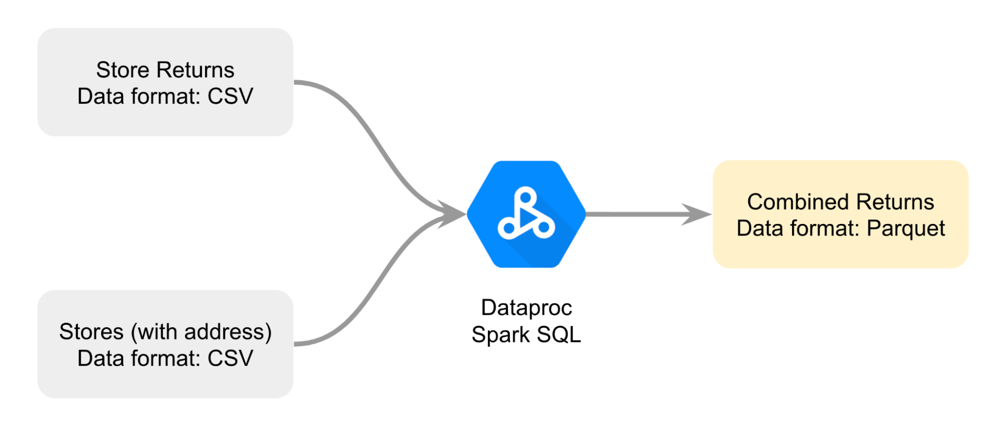
This is the data that you'll use as the basis of your comparison.

Here's how you'll do this task: First, you'll open a Jupyter notebook on a Dataproc cluster. Next, you'll follow the instructions in the notebook to join the two CSV files to create a Parquet file. Then , you'll load the data from the Parquet file stored into a Cloud Storage bucket into a BigQuery standard table to analyze the data. Finally, you'll reference the same Parquet into a Jupyter notebook on a Dataproc cluster to compare data analysis using BigQuery to data analysis using Dataproc and Spark.

Setup

Before you click Start Lab

Read these instructions. Labs are timed and you cannot pause them. The timer, which starts when you click Start Lab, shows how long Google Cloud resources will be made available to you.

This practical lab lets you do the activities yourself in a real cloud environment, not in a simulation or demo environment. It does so by giving you new, temporary credentials that you use to sign in and access Google Cloud for the duration of the lab.

To complete this lab, you need:

• Access to a standard internet browser (Chrome browser recommended).

Note: Use an Incognito or private browser window to run this lab. This prevents any conflicts between your personal account and the Student account, which may cause extra charges incurred to your personal account.

• Time to complete the lab---remember, once you start, you cannot pause a lab.

Note: If you already have your own personal Google Cloud account or project, do not use it for this lab to avoid extra charges to your account.

How to start your lab and sign in to the Google Cloud console

1. Click the Start Lab button. On the left is the Lab Details panel with the following:

   • Time remaining
   • The Open Google Cloud console button
   • The temporary credentials that you must use for this lab
   • Other information, if needed, to step through this lab
   Note: If you need to pay for the lab, a pop-up opens for you to select your payment method.

2. Click Open Google Cloud console (or right-click and select Open Link in Incognito Window) if you are running the Chrome browser. The Sign in page opens in a new browser tab.

   Tip: You can arrange the tabs in separate, side-by-side windows to easily switch between them.

   Note: If the Choose an account dialog displays, click Use Another Account.

3. If necessary, copy the Google Cloud username below and paste it into the Sign in dialog. Click Next.

{{{user_0.username | "Google Cloud username"}}}

You can also find the Google Cloud username in the Lab Details panel.

4. Copy the Google Cloud password below and paste it into the Welcome dialog. Click Next.

{{{user_0.password | "Google Cloud password"}}}

You can also find the Google Cloud password in the Lab Details panel.

Important: You must use the credentials the lab provides you. Do not use your Google Cloud account credentials. Note: Using your own Google Cloud account for this lab may incur extra charges.

5. Click through the subsequent pages:
   • Accept the terms and conditions
   • Do not add recovery options or two-factor authentication (because this is a temporary account)
   • Do not sign up for free trials

After a few moments, the Console opens in this tab.

Note: You can view the menu with a list of Google Cloud Products and Services by clicking the Navigation menu at the top-left. Note: After you click Start Lab, the time to provision the lab resources is provided. However, it may take a bit longer than indicated.

Task 1. Open JupyterLab on a Dataproc cluster

JupyterLab can be used to create, open, and edit Jupyter notebooks on a Dataproc cluster. This allows you to take advantage of the cluster's resources, such as its high performance and scalability, and to run your notebooks faster and on larger datasets. You can also use JupyterLab to collaborate with others on projects.

In this task, you'll open an existing Dataproc cluster in Dataproc and navigate to JupyterLab to locate the Jupyter notebooks that you'll use to complete the remaining tasks for this lab.

1. In the Google Cloud console title bar, type "Dataproc" into the Search field and press ENTER.
2. From the search results, select Dataproc.
3. On the Clusters page, click the name of the cluster listed, mycluster.
4. On the Cluster details tabbed page, select the Web Interfaces tab.
5. Under the Component gateway section, click the JupyterLab link.

Note: Be careful not to confuse the JupyterLab link with the Jupyter link.

The JupyterLab environment opens in a new browser tab.

6. Locate the C2M4-1 Combine and Export.ipynb file listed in the left sidebar.

Task 2. Combine the data and export Parquet files

To help Meredith identify the locations and markets, Meredith needs information about each return and the physical address where the return was made. But this information is in two separate CSV files.

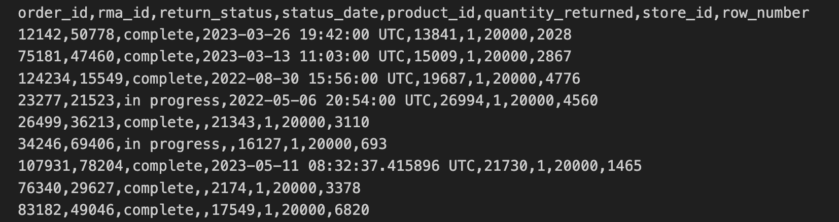
The store returns data has been exported from stores in CSV format and copied to a Cloud Storage bucket. This data includes the order_id, rma_id, return_status, status_date, product_ied, quantity_returned, store_id.

The first 10 lines of the store returns CSV contain the following:

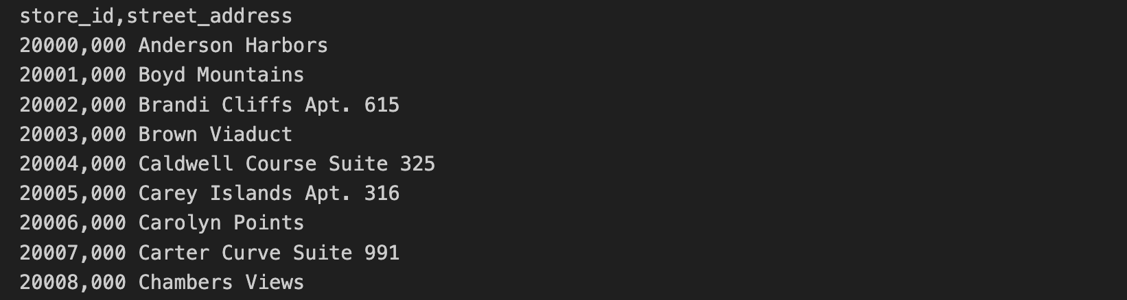
The store address data is included in a separate CSV file. This data includes the store_id and the street_address.

The first 10 lines of the store address CSV contain the following:

In this task, you'll run the SQL queries and Python commands contained in the C2M4-1 Combine and Export.ipynb file, to join the two CSV files. The combined files will be stored as a Parquet file.

1. In the left sidebar, double click the C2M4-1 Combine and Export.ipynb file to open it in the JupyterLab environment.

Note: If the Select Kernel dialog box opens, select PySpark and click the Select button. For more information on running code in Jupyter Notebook, refer to the Jupyter Notebook documentation.

Next, follow the instructions in the notebook and execute the code in each of the cells.

2. Click each cell in the notebook, and click the Run the selected cells and advance icon () to execute each cell. Alternatively, press SHIFT+ENTER to run the code. Cells that depend on a previous cell's output MUST be run in order. If you make a mistake and run a cell out of order, click the Refresh button () in the notebook toolbar to restart the kernel.

Note: The cells in the notebook must be run in order to execute properly. If you receive an error message when running a cell in the notebook, make sure that each cell has been executed and try re-running the entire notebook to clear the error.

3. Explore the outputs from each cell in the notebook. The two CSV files are now joined, and the Parquet file, you'll use in the next task, has been automatically created.

A Spark session in Dataproc is a way to connect to a Dataproc cluster and run Spark applications. It is the main way to start Spark applications and create Dataframes. Dataframes are tables that Spark can process and run queries. Using Spark, you can also read and write data to different storage systems, such as Google Cloud Storage or BigQuery.

Note: Dataproc can also process queries saved in text files, which is the typical solution for automated processes. Using a notebook is a standard approach during development and data exploration.

In this notebook, you created a Spark session and loaded the store returns data from a CSV file to a DataFrame, a table used in Spark. Next, you loaded the store addresses from a second CSV file and joined the two Dataframes and exported the single, joined table as a Parquet file. Finally, you used a query to modify the name of one of the columns.

Hint: Keep the notebook with the outputs open while you answer the questions below.

Click Check my progress to verify that you have completed this task correctly. Combine the data and export Parquet files

Task 3. Query data in BigQuery

Now that the combined Parquet file is created and stored in a Cloud Storage bucket, you are ready to compare the two ways to run analytics: one centered in BigQuery and one centered in Dataproc and Spark.

Start with BigQuery, a data warehouse that uses the BigQuery engine to execute queries and analyze data.

In the last task, you created a Parquet file and stored it in a Cloud Storage bucket. To access this data in BigQuery, you have two choices: an external table or a standard table. External tables reference data that is stored outside of BigQuery, such as in Google Cloud Storage. Standard tables store a copy of the data directly in BigQuery.

Artem told you that standard tables are often the more efficient choice for working with big data, since the data can be queried and processed quickly. So, you decide that a standard table is the best choice for this task.

In this task, you'll load the Parquet file into a standard table in BigQuery and run a query using GoogleSQL, the SQL dialect used in the BigQuery environment. Then, you'll answer questions to make sure you have the information you need to compare BigQuery with Dataproc and Spark in the next task.

1. Return to the Google Cloud console browser tab (where you should still have the Dataproc page open), while keeping the JupyterLab browser tab open.

2. In the Google Cloud console Navigation menu (), click BigQuery > BigQuery Studio. BiqQuery Studio is the primary way to write and run queries in BigQuery.

Note: The Welcome to BigQuery in the Cloud Console message box may appear, providing links to the quickstart guide and the release notes for UI updates. Click Done to proceed.

3. In the Query Editor, click the Compose new query (+) icon to open a new Untitled tab.

4. Copy the following query into Untitled tab:

LOAD DATA OVERWRITE thelook_gcda.product_returns_to_store FROM FILES ( format="PARQUET", uris=["gs://{{{project_0.project_id | "PROJECT_ID"}}}/store_returns_output/store_returns.parquet/*.parquet"] ) ;

This query imports the Parquet file into BigQuery.

5. Click Run.

A URI (Uniform Resource Identifier) is the path to a file in a Cloud Storage bucket. A collection of URIs can be provided as input to the LOAD DATA command by enclosing the URIs in square brackets []. This indicates that the value is an array of URIs.

The URI always starts with gs://, indicating that it is a resource in Cloud Storage. The URI provided in the example above filters for files with a .parquet extension, as it ends with *.parquet. The * symbol is a wildcard, meaning any string.

This query returns all files in the path gs:///store_returns_output/store_returns.parquet/ that have any name that ends with .parquet, and loads the data into the store_returns table.

6. Copy the following query into the Query Editor:

SELECT count(*) FROM thelook_gcda.product_returns_to_store;

This query returns the number of rows in the 'thelook_gcda.product_returns_to_store' table.

7. Click Run.

By default, when you run a query in the BigQuery Studio, it is executed using the GoogleSQL dialect. GoogleSQL is a superset of the standard SQL dialect, meaning it includes all standard SQL queries and additional extensions that make it easier to work with large amounts of data and complex data types in BigQuery.

8. Copy the following query into the Query Editor:

SELECT substring(status_date, 1, 7) as year_month, return_status, count(order_id) as order_count FROM thelook_gcda.product_returns_to_store GROUP BY year_month, return_status;

This query displays the number of returns received by month and by status.

9. Click Run.

Note: The year_month column might have null values in the output.

Click  Check my progress  to verify that you have completed this task correctly.

Query data in BigQuery

Task 4. Query data in Dataproc and Spark

Now that you have completed your analysis in BigQuery, you're ready to explore analysis centered in Dataproc and Spark.

Spark is the main data processing engine for analyzing data with Dataproc. Dataproc automatically manages the Spark cluster and comes pre-installed with Spark, making it a convenient and powerful choice for data analysis.

Spark also uses its own SQL dialect, Spark SQL. Like GoogleSQL, Spark SQL is a SQL dialect. Spark SQL is a distributed SQL dialect, which means it can query and analyze data distributed across multiple machines in the Spark cluster.

To run Spark SQL queries with Dataproc and Spark, you'll use a Jupyter Notebook. This interactive environment allows you to write code and easily display its output.

In this task, you'll run Spark SQL queries on the Parquet file that is referenced from the Cloud Storage bucket. Then you'll answer questions that will help you complete the comparison of two ways to run analytics: one centered in BigQuery and one centered in Dataproc and Spark.

1. Return to the JupyterLab tab in your browser.

2. Double click the C2M4-2 Query Store Data with Spark SQL.ipynb file to open it in the JupyterLab environment.

Follow the instructions in the notebook and execute the code in each of the cells.

3. Click each cell in the notebook, and click Run or press SHIFT+ENTER to run the code.

4. Explore the outputs from the Spark SQL queries in the notebook.

In this notebook, you first created a Spark session. Then, you referenced the data from the Parquet files in Cloud Storage using the The iPython notebook and populated a DataFrame. Next, you created a view so the DataFrame could be used with Spark SQL. Then, you ran a Spark SQL query that returned the top three rows from the DataFrame. Finally, you ran the same query as you ran in BigQuery in the previous step.

Click  Check my progress  to verify that you have completed this task correctly.

Query data in Dataproc and Spark

Task 5. Stop the cluster

As a best practice, before exiting the environment, make sure to stop the cluster.

Note: Leaving clusters running uses resources and may cause you to incur extra cost.

1. Return to the BigQuery tab in your browser.
2. In the Google Cloud console title bar, type Dataproc into the Search field.
3. Select Dataproc from the search results. The Clusters page opens.
4. In the cluster list, select the checkbox next to mycluster.
5. In the Action bar, click Stop.

Summary

Review the following table that summarizes the differences between data analysis with BigQuery and data analysis with Dataproc and Spark covered in this lab.

	Task 3	Task 4
Central product	BigQuery	Dataproc
Data Processing Engine	BigQuery	Spark
Data location	BigQuery Standard Table	Parquet File in GCS
SQL Dialect	GoogleSQL	Spark SQL
Development Environment	BigQuery Studio	Jupyter Notebooks

Conclusion

Great work!

You've successfully collected and processed the data needed for Meredith's report and used the combined data to compare two approaches to running analytics: one centered in BigQuery, a product you're familiar with, and one centered in Dataproc and Spark.

First, you opened a Jupyter notebook on an existing Dataproc cluster.

Then, you followed the instructions in the notebook to join two CSV files containing returns and address data to create a combined Parquet file and store the Parquet file in a Cloud Storage bucket.

Taking Artem's advice, you then used the combined Parquet file to compare analyzing data using BigQuery and Dataproc and Spark to learn more about their data processing engines, SQL dialects, data locations, and development environment.

You're well on your way to understanding how to use Dataproc and Spark to work with large datasets.

End your lab

Before you end the lab , make sure you're satisfied that you've completed all the tasks. When you're ready, click End Lab and then click Submit.

Ending the lab will remove your access to the lab environment, and you won't be able to access the work you've completed in it again.